TGA-BeFlat®
TGA-BeFlat® is a mathematical procedure allowing for the removal from TGA measurement of the contribution of physical phenomena, thus influencing the measured TGA value. These phenomena are: buoyancy effect and friction force from the vertically moving gas. This force is a function of the gas flow and the temperature-dependent gas viscosity. Application of TGA-BeFlat® means: If a sample is measured in flowing gas without a separate baseline measurement, the software calculates the baseline and sub-tracts it from the sample measurement. The usual procedure for removing these physical phenomena is to measure a baseline and to subtract it from the sample measurement.
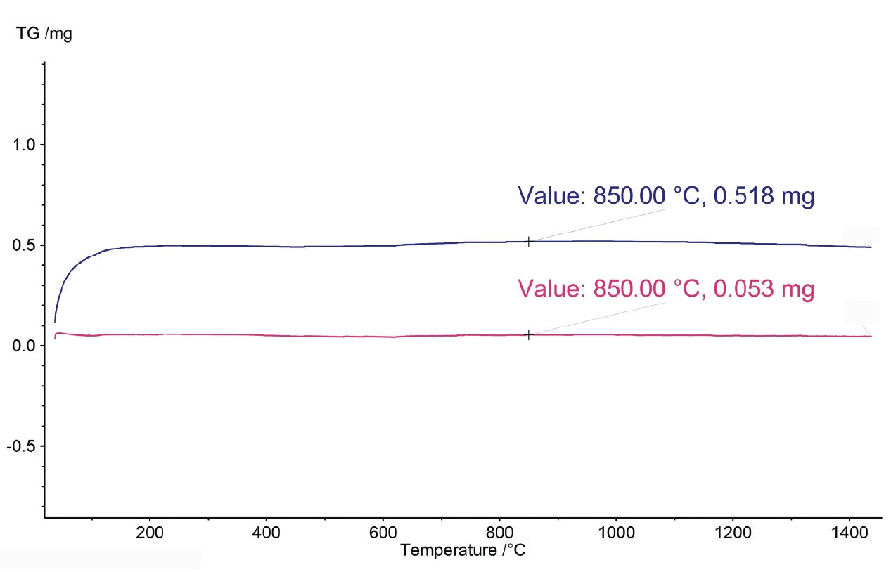
However, if a sample should be measured under gas flow conditions without a separate baseline measurement, the software must calculate the baseline and subtract it from the sample measurement. Figure 1 demonstrates the effectiveness of TGA-BeFlat®. The measurement was carried out using the STA 449 F5 Jupiter® with empty crucibles (without sample and reference sample) at a heating rate of 10 K/min. The blue curve is the measured data including the influence of the physical effects described above. The red curve corresponds to the BeFlat®-corrected data, where the baseline is calculated and subtracted from the measurement curve. For convenience, the software solution TGA-BeFlat® is now included in the Proteus® software of the TG 209 F1 Libra® and STA 449 F5 Jupiter® instruments; optionally also avail-able for other instruments.
DSC-BeFlat®
DSC-BeFlat® is a mathematical procedure allowing for the removal from a DSC measurement of the contribution of the physical phenomena, thus influencing the measured DSC value. Some of these phenomena are: non-symmetry of the DSC sensor, differing leves of thermal contact between the sensor and crucibles for the sample side, and reference side and different crucible masses for the sample and reference. It is not used as often in thermogravimetry, but just as with TGA, these physical phenomena are usually removed by measurement of the baseline and its subtraction from the sample measurement. Again, a sample measurement without a baseline measurement requires the software to calculate a baseline and subtract it from the sample measurement. The two methods of Standard BeFlat® and Advanced BeFlat® generally do the same: calculate the baseline and subtract it. The difference between these two methods is the way the baseline is calculated.
Standard DSC BeFlat®
Mathematical Approach:
The DSC-BeFlat® software add-on for the correction of temperature- and heating rate-dependent DSC baseline deviations over a multi-dimensional polynomial function is designed to help achieve the highest possible baseline stability with minimal curvature across a broad tempera-ture range. It is known that a DSC measurement depends on the tem-perature and heating rate. The most common dependence can be presented as the polynomial of two variables: tem-perature (T) and heating rate (HR).

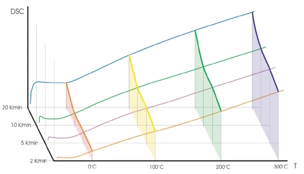
In order to find the unknown coefficients ai,k, it is necessary to carry out several measurements at different heating rates for the same temperature range, which must be at least several hundred K in width. Figure 2 shows that the baseline depends on the heating rate for each temperature.
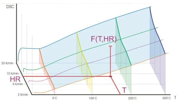
Equation (1) creates a two-dimensional surface as a function of temperature and heating rate. This surface is marked with blue in fig. 3. This function is enabled only in the range of the measured temperatures and heating rates: here, temperatures from 0 to 300°C and heating rates from 2 to 20 K/min.
Depending on the instrument, Standard BeFlat® may either require several heating segments in one measurement (DSC) or several independent measurements, as in the case of STA.
Advanced BeFlat®
Physical Approach:
The physical model for the heat flow is described mathematically for the system containing furnace, sensor with two positions and two crucibles. The values of the ther-mal resistance inside the sensor and thermal resistances between the crucible and sensor are unknown. The contribution of the mass difference between the sample crucible and reference crucible is proportional to the heating rate, but the proportionality coefficient is unknown as well. In order to find these temperature-dependent unknown parameters, it is necessary to carry out two calibration measurements: a first heating with only one empty crucible on the reference side (and no crucible on the sample side) and the second measurement with two empty crucibles.
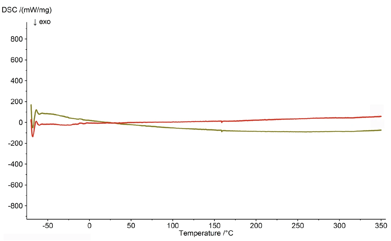
From these two measurements, all unknown parameters are found as a function of temperature. Figure 4 represents an example of Advanced DSC-BeFlat® for a heating segment (two empty crucibles, no sample); the green curve is the measured data. The red curve is the BeFlat®-corrected data where the baseline is calculated and subtracted.
Conclusion
The BeFlat® and Advanced DSC-BeFlat® software features are integrated in the Proteus® software as of versions 7.0 and 7.1, respectively. Both allow for effective and precise measurements without the necessity of additional baseline measurements.