Quelle est la méthode la mieux adaptée à mon échantillon particulier ?
Les méthodes présentées pour la conductivité et la diffusivité thermiques diffèrent les unes des autres principalement en ce qui concerne la géométrie recommandée de l'échantillon et les plages de diffusivité et de conductivité thermiques réalisables.
Le tableau 1 donne un aperçu des tailles d'échantillon appropriées.
| ACL | BPE | hFM* | ||
|---|---|---|---|---|
| Forme de l'échantillon | Rond ou rectangulaire | Carré | Rond ou rectangulaire | |
| Nombre de pièces par échantillon | 1 | 2 | 1 | |
| Diamètre et/ou longueur des bords | 6 mm à 25,4 mm | 300 mm x 300 mm | 150 mm x 150 mm à 300 mm x 300 mm (ou 305 mm x 305 mm à 610 mm x 610 mm) | |
| Épaisseur maximale | 6 mm | 100 mm | 100 mm (ou 200 mm) | |
| Épaisseur min | 0.01 mm, en fonction des propriétés de l'échantillon | Environ 1 mm, en fonction de l'échantillon | Environ 5 mm |
* Trois modèles de HFM sont disponibles pour différentes tailles d'échantillons
Tableau:1 Géométries d'échantillons établies
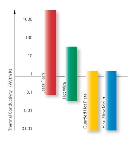
En raison de leur capacité d'échantillonnage relativement large, les HFM (Heat Flow Meters) et les GHP (Guarded Hot Plates) - les méthodes de détermination directe de la Conductivité thermiqueLa conductivité thermique (λ avec l'unité W/(m-K)) décrit le transport d'énergie - sous forme de chaleur - à travers un corps de masse sous l'effet d'un gradient de température (voir fig. 1). Selon la deuxième loi de la thermodynamique, la chaleur s'écoule toujours dans la direction de la température la plus basse.conductivité thermique - sont principalement utilisées pour les matériaux d'échantillonnage inhomogènes (matériaux d'isolation).
Les appareils à laser ou à flash lumineux (LFA) sont configurés pour traiter des échantillons de taille beaucoup plus petite. Les échantillons standard ont une taille de 12,7 mm et une épaisseur de 2 à 3 mm.
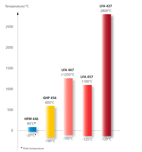
La figure 1 donne un aperçu des différentes conductivités thermiques en fonction de la méthode utilisée et la figure 2 pour les plages de température.