Advanced Models Needed for Laser Flash Analysis
For laser flash analysis, advanced models are needed because real experiments never meet the ideal assumptions built into the basic Parker model. Therefore, uncorrected data provides incorrect values for Thermal DiffusivityThermal diffusivity (a with the unit mm2/s) is a material-specific property for characterizing unsteady heat conduction. This value describes how quickly a material reacts to a change in temperature.thermal diffusivity and derived conductivity/specific heat.
The classic Parker evaluation assumes the following:
- Perfectly AdiabaticAdiabatic describes a system or measurement mode without any heat exchange with the surroundings. This mode can be realized using a calorimeter device according to the method of accelerating rate calorimetry (ARC). The main purpose of such a device is to study scenarios and thermal runaway reactions. A short description of the adiabatic mode is “no heat in – no heat out”.adiabatic conditions (no heat loss to the surroundings).
- Instantaneous, spatially uniform energy input at the front face;
- One-dimensional heat flow through a homogeneous, opaque sample with a perfect surface coating.
Under these assumptions, the simple relation α = 0.1388 d2/t1/2 (thickness d, half‑rise time t1/2) is valid.
In practice, none of these assumptions are strictly true, particularly at higher temperatures or when working with thin or translucent samples.
Several corrections and advanced models are implemented in the software for Laser Flash Analysis (LFA) to achieve the highest accuracy. To improve the fit and achieve the best results, all models are available by default with pulse and baseline corrections. The user is free to turn off those corrections to measurement signals. In addition all models take heat loss into account.
Improvements on Pulse Correction That Impact All Models
Pulse (finite-pulse-width) correction is required in laser flash analysis because the laser pulse is not truly instantaneous. This non-ideality directly distorts the time-temperature curve used to calculate Thermal DiffusivityThermal diffusivity (a with the unit mm2/s) is a material-specific property for characterizing unsteady heat conduction. This value describes how quickly a material reacts to a change in temperature.thermal diffusivity.
In the latest analysis software version, a refined pulse correction enables precise analysis of samples requiring exceptional time resolution. This is advantageous for thin, highly conductive samples or when the light pulse overlaps significantly with the thermal response.
The user can select among:
- Equivalent square
- Gravity center
- Double exponential pulse correction
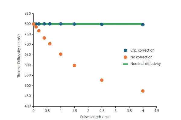
Applying pulse correction influences the model fit, as demosntrated by simulations for materials with high Thermal DiffusivityThermal diffusivity (a with the unit mm2/s) is a material-specific property for characterizing unsteady heat conduction. This value describes how quickly a material reacts to a change in temperature.thermal diffusivity (see below). The correction’s relevance appears when simulating various pulse lengths: without correction, calculated diffusivity decreases with longer pulses, while exponential correction keeps it nearly constant.
This allows fast determination of Thermal DiffusivityThermal diffusivity (a with the unit mm2/s) is a material-specific property for characterizing unsteady heat conduction. This value describes how quickly a material reacts to a change in temperature.thermal diffusivity regardless of pulse length.

The Importance of Pulse Correction
The importance of the pulse correction becomes more apparent when sumulating different pulse lengths as shown below.
For uncorrected data, the calculated Thermal DiffusivityThermal diffusivity (a with the unit mm2/s) is a material-specific property for characterizing unsteady heat conduction. This value describes how quickly a material reacts to a change in temperature.thermal diffusivity decreases with increasing pulse length. When an exponential pulse correction is applied, however, the diffusivity remains almost constant over the simulated range of pulse lengths. This correction enables any user to rapidly evaluate the real diffusivities of samples.